Visualizing the Internet (2026)
This post is part of the internet-map series.
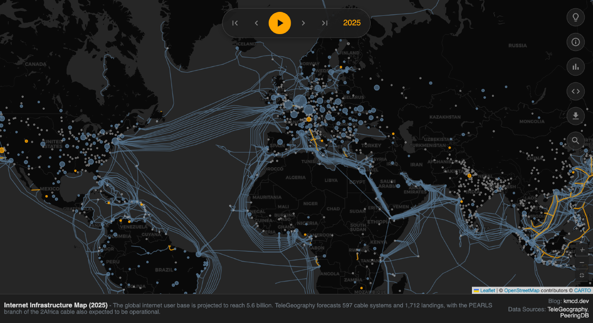
For the past few years, I’ve been trying to make the physical reality of the Internet visible with my Internet Infrastructure Map. This map shows the network of undersea fiber-optic cables along with peering bandwidth, grouped by city. I update the map annually, but I don’t want to just pull the latest data and call it a day. In this post I discuss how the map evolved this year and what I did to make it happen, but you can skip to the good part by viewing it here: map.kmcd.dev.
For the 2026 edition, I wanted to better answer the question: where does the Internet actually live? By layering on BGP routing tables alongside physical infrastructure data, I’m now closer to answering that question.
The result is a concept I call “Logical Dominance.” Each city’s dominance is calculated by summing total address space of IPv4 subnets that are “homed” in that city. How can I tell where IP addresses are homed? This required analyzing global routing tables to trace IP ownership back to specific geographies. Read on to find out how I accomplished this!


How the Internet Routes Traffic
Previous versions of the map focused on physical infrastructure: cables and exchange points. The physical path is only half the story. To understand how data moves, we have to look at BGP (Border Gateway Protocol).
BGP is the protocol that distinct networks, known as Autonomous Systems (AS), use to announce which IP addresses they own and how to reach them. If the cables are the hardware, BGP is the software that ties the Internet together. Cloudflare has an excellent primer.
When you load a webpage, your request doesn’t just “know” the path. Your ISP’s routers consult the global BGP routing table to decide the best next hop. Visualized, it looks a little bit like this:

In this state, the route from Router -> Netstream (AS8283) -> Google (AS15169) was chosen, at least for now. The underlying routes of the global Internet change thousands of times per second, constantly reshaping the topology.
Sources of BGP Data
To visualize this layer, we need access to routing tables. I explored three ways to get this data, each with its own trade-offs between real-time visibility and historical context.
Query a Looking Glass
We can connect to public routers via projects like University of Oregon Route Views. These allow you to telnet in and run standard CLI commands like show ip bgp to see exactly what a backbone router sees.
BGP routes for 8.8.8.8 (click to expand)View on GitHub
$ telnet route-views.routeviews.org 23
**********************************************************************

                    RouteViews BGP Route Viewer
                    route-views.routeviews.org

 RouteViews data is archived on https://archive.routeviews.org

 This hardware is part of a grant by the NSF.

 Please contact [email protected] if you have questions, or
 if you wish to contribute your view.

 This router has views of full routing tables from several ASes.

 The current list of all RouteViews peers is at
   https://www.routeviews.org/peers/peering-status.html

 NOTE: If you are using macOS and seeing the error message
 "no default Kerberos realm" when logging in, you may want to
 add "default unset autologin" to your ~/.telnetrc

 To login, use the username "rviews".

**********************************************************************


User Access Verification

Username: rviews
route-views>show ip bgp 8.8.8.8
BGP routing table entry for 8.8.8.0/24, version 941738530
Paths: (16 available, best #15, table default)
  Not advertised to any peer
  Refresh Epoch 1
  4826 15169
    114.31.199.16 from 114.31.199.16 (114.31.199.16)
      Origin IGP, localpref 100, valid, external
      Community: 4826:5203 4826:6510 4826:52032
      path 7F168F059710 RPKI State valid
      rx pathid: 0, tx pathid: 0
  Refresh Epoch 1
  57866 15169
    37.139.139.17 from 37.139.139.17 (37.139.139.17)
      Origin IGP, metric 0, localpref 100, valid, external
      Community: 57866:200 65102:56393 65103:1 65104:31
      unknown transitive attribute: flag 0xE0 type 0x20 length 0x30
        value 0000 E20A 0000 0065 0000 00C8 0000 E20A
              0000 0066 0000 DC49 0000 E20A 0000 0067
              0000 0001 0000 E20A 0000 0068 0000 001F

      path 7F15A63304E8 RPKI State valid
      rx pathid: 0, tx pathid: 0
  Refresh Epoch 1
  6939 15169
    64.71.137.241 from 64.71.137.241 (216.218.253.53)
      Origin IGP, localpref 100, valid, external
      path 7F1555102CB8 RPKI State valid
      rx pathid: 0, tx pathid: 0
  Refresh Epoch 1
  20130 6939 15169
    140.192.8.16 from 140.192.8.16 (140.192.8.16)
      Origin IGP, localpref 100, valid, external
      path 7F1588A8BD60 RPKI State valid
      rx pathid: 0, tx pathid: 0
  Refresh Epoch 1
  3333 1257 15169
    193.0.0.56 from 193.0.0.56 (193.0.0.56)
      Origin IGP, localpref 100, valid, external
      Community: 1257:50 1257:51 1257:3528
      path 7F16B16DD098 RPKI State valid
      rx pathid: 0, tx pathid: 0
  Refresh Epoch 1
  7018 15169
    12.0.1.63 from 12.0.1.63 (12.0.1.63)
      Origin IGP, localpref 100, valid, external
      Community: 7018:2500 7018:37232
      path 7F1626828FD8 RPKI State valid
      rx pathid: 0, tx pathid: 0
  Refresh Epoch 1
  20912 15169
    77.39.192.30 from 77.39.192.30 (77.39.192.1)
      Origin IGP, localpref 100, valid, external
      Community: 20912:65002 20912:65022
      path 7F15D19801C0 RPKI State valid
      rx pathid: 0, tx pathid: 0
  Refresh Epoch 1
  3356 15169
    4.68.4.46 from 4.68.4.46 (4.69.184.201)
      Origin IGP, metric 0, localpref 100, valid, external
      Community: 3356:3 3356:86 3356:576 3356:666 3356:901 3356:2012
      path 7F1679EB7640 RPKI State valid
      rx pathid: 0, tx pathid: 0
  Refresh Epoch 1
  3549 3356 15169
    208.51.134.254 from 208.51.134.254 (67.16.168.191)
      Origin IGP, metric 0, localpref 100, valid, external
      Community: 3356:3 3356:22 3356:86 3356:575 3356:666 3356:901 3356:2011 3549:2581 3549:30840
      path 7F16C7D32728 RPKI State valid
      rx pathid: 0, tx pathid: 0
  Refresh Epoch 1
  101 15169
    209.124.176.223 from 209.124.176.223 (209.124.176.224)
      Origin IGP, localpref 100, valid, external
      Community: 101:20400 101:22200 101:24100
      path 7F1648388978 RPKI State valid
      rx pathid: 0, tx pathid: 0
  Refresh Epoch 1
  1351 15169
    132.198.255.253 from 132.198.255.253 (132.198.255.253)
      Origin IGP, localpref 100, valid, external
      path 7F15C90D61B8 RPKI State valid
      rx pathid: 0, tx pathid: 0
  Refresh Epoch 1
  3257 15169
    89.149.178.10 from 89.149.178.10 (213.200.83.26)
      Origin IGP, metric 10, localpref 100, valid, external
      Community: 3257:8052 3257:30306 3257:50001 3257:54900 3257:54901
      path 7F154665E650 RPKI State valid
      rx pathid: 0, tx pathid: 0
  Refresh Epoch 1
  2497 15169
    202.232.0.2 from 202.232.0.2 (58.138.96.254)
      Origin IGP, localpref 100, valid, external
      path 7F1660B0A1C8 RPKI State valid
      rx pathid: 0, tx pathid: 0
  Refresh Epoch 2
  3303 15169
    217.192.89.50 from 217.192.89.50 (138.187.128.158)
      Origin IGP, localpref 100, valid, external
      Community: 3303:1004 3303:1007 3303:3067
      path 7F16E10C0508 RPKI State valid
      rx pathid: 0, tx pathid: 0
  Refresh Epoch 1
  8283 15169
    94.142.247.3 from 94.142.247.3 (94.142.247.3)
      Origin IGP, localpref 100, valid, external, best
      Community: 8283:1 8283:101 8283:102
      unknown transitive attribute: flag 0xE0 type 0x20 length 0x30
        value 0000 205B 0000 0000 0000 0001 0000 205B
              0000 0005 0000 0001 0000 205B 0000 0005
              0000 0002 0000 205B 0000 0008 0000 001A

      path 7F16DC0E5B28 RPKI State valid
      rx pathid: 0, tx pathid: 0x0
  Refresh Epoch 1
  49788 12552 15169
    91.218.184.60 from 91.218.184.60 (91.218.184.60)
      Origin IGP, localpref 100, valid, external
      Community: 12552:10000 12552:14000 12552:14100 12552:14101 12552:24000
      Extended Community: 0x43:100:0
      path 7F15CAD0C378 RPKI State valid
      rx pathid: 0, tx pathid: 0
route-views>⏎
These paths often carry metadata called BGP Communities. These are optional tags that networks use to signal things like geographic origin or peering policy. While perfect for debugging today’s Internet, this approach lacks historical context; you can’t telnet into 2012 to check a routing table from 14 years ago.
Subscribe to a Stream
For real-time views, services like RIPE RIS Live aggregate BGP data from global collectors and stream it over a public WebSocket. You can watch the Internet “breathe” as routes are announced and withdrawn thousands of times per second. This is fascinating for a live dashboard, but useless for backfilling history.
Here’s an example script consuming this stream:go/stream_bgp/main.go (click to expand)View on GitHub
package main

import (
	"fmt"
	"log"
	"os"
	"os/signal"
	"time"

	"github.com/gorilla/websocket"
)

// RIPE RIS Live WebSocket URL
const risLiveURL = "wss://ris-live.ripe.net/v1/ws/?client=kmcd-internet-map"

// Message defines the structure of the JSON messages we receive
type Message struct {
	Type string                 `json:"type"`
	Data map[string]interface{} `json:"data"`
}

func main() {
	// Handle Ctrl+C gracefully
	interrupt := make(chan os.Signal, 1)
	signal.Notify(interrupt, os.Interrupt)

	fmt.Printf("Connecting to %s...\n", risLiveURL)

	c, _, err := websocket.DefaultDialer.Dial(risLiveURL, nil)
	if err != nil {
		log.Fatal("dial:", err)
	}
	defer c.Close()

	// Subscribe to the firehose (all messages)
	// You can filter this! e.g., {"host": "rrc21"} for a specific collector
	subscribeMsg := map[string]interface{}{
		"type": "ris_subscribe",
		"data": map[string]interface{}{
			"moreSpecific": true,
			"type":         "UPDATE", // Only show route updates
		},
	}

	if err := c.WriteJSON(subscribeMsg); err != nil {
		log.Fatal("subscribe:", err)
	}

	fmt.Println("Connected! Streaming global BGP updates...")
	fmt.Println("------------------------------------------------")

	done := make(chan struct{})

	go func() {
		defer close(done)
		for {
			var msg Message
			err := c.ReadJSON(&msg)
			if err != nil {
				log.Println("read:", err)
				return
			}

			// We only care about BGP UPDATE messages
			if msg.Type == "ris_message" {
				path := msg.Data["path"]
				prefix := msg.Data["announcements"]

				// Handle withdrawals (routes being removed)
				if prefix == nil {
					prefix = "WITHDRAWAL"
				}

				// Print the timestamp, the route prefix, and the AS path
				fmt.Printf("[%s] Prefix: %v | Path: %v\n",
					time.Now().Format("15:04:05"),
					prefix,
					path,
				)
			}
		}
	}()

	// Wait for interrupt
	<-interrupt
	fmt.Println("\nDisconnecting...")
	err = c.WriteMessage(websocket.CloseMessage, websocket.FormatCloseMessage(websocket.CloseNormalClosure, ""))
	if err != nil {
		log.Println("write close:", err)
		return
	}
	select {
	case <-done:
	case <-time.After(time.Second):
	}
}
The output looks like this:Websocket Stream Output (click to expand)View on GitHub
Connecting to wss://ris-live.ripe.net/v1/ws/?client=kmcd-internet-map...
Connected! Streaming global BGP updates...
------------------------------------------------
[22:52:35] Prefix: [map[next_hop:2001:7f8:24::b1 prefixes:[2804:70c0::/32]]] | Path: [58057 6939 22381 1031 263444 22381 270746]
[22:52:35] Prefix: [map[next_hop:2001:7f8:24::aa,fe80::8a7e:25ff:fed3:420b prefixes:[2a13:9404::/32]]] | Path: [6939 215120 34689]
[22:52:35] Prefix: [map[next_hop:2001:7f8:24::aa,fe80::470:71ff:fec5:b6ad prefixes:[2a14:7c0:1740::/48 2a10:ccc7:b110::/44]]] | Path: [196621 6939 215120 214497 6204 215120 214497]
[22:52:35] Prefix: [map[next_hop:2001:7f8:24::aa,fe80::224:38ff:fea4:a907 prefixes:[2a14:7c0:1740::/48 2a10:ccc7:b110::/44]]] | Path: [29691 6939 215120 214497 6204 215120 214497]
[22:52:35] Prefix: [map[next_hop:91.206.52.177 prefixes:[2a10:ccc7:b110::/44 2a14:7c0:1740::/48]]] | Path: [58057 6939 215120 214497 6204 215120 214497]
[22:52:35] Prefix: [map[next_hop:2001:7f8:24::b1 prefixes:[2803:5d10::/32]]] | Path: [58057 6939 3356 28343 272053]
[22:52:35] Prefix: [map[next_hop:2001:7f8:24::aa,fe80::8a7e:25ff:fed3:420b prefixes:[2a14:7c0:1740::/48 2a10:ccc7:b110::/44]]] | Path: [6939 215120 214497]
[22:52:35] Prefix: [map[next_hop:2001:7f8:24::aa,fe80::470:71ff:fec5:b6ad prefixes:[2a13:9404::/32]]] | Path: [196621 6939 215120 34689]
2026/02/09 22:52:35 read: websocket: close 1000 (normal)
Download Historical Snapshots
To build the historical model, I processed raw RIB (Routing Information Base) files. These are snapshots of the entire routing table as seen by a backbone router at a specific moment in time. Because BGP is a “chatter” protocol that only announces changes, these full table dumps are essential for reconstructing the state of the Internet at any point in the past.
I specifically fetched snapshots from February 1st at 12:00 UTC for every year in my timeline. To ensure a comprehensive view, I aggregated data from multiple global collectors maintained by the University of Oregon Route Views project.
Other excellent resources for this kind of data include:
- RIPE RIS (Routing Information Service): Provides high-fidelity snapshots from a dense network of collectors, primarily in Europe.
- CAIDA BGP Stream: A framework for analyzing both real-time and historical data from various sources.
How BGP Shapes the Global Internet Map
For this edition, I processed over 15 years of BGP snapshots and PeeringDB archives to build the Logical Dominance model. Reconstructing this history was easily the hardest part of the project. I quickly realized that reliable archival data for physical peering effectively vanishes before 2010, which set a hard limit on how far back I could take the timeline.
Defining Logical Dominance
Logical Dominance is calculated by summing the number of unique IPv4 addresses originated by an ASN and attributed to a given city. Overlapping prefixes are deduplicated using longest-prefix normalization so that no address space is counted twice.
The Scaling Problem: Why not IPv6?
You might notice this model focuses entirely on IPv4. While IPv6 is the future of the protocol, its sheer scale currently breaks the “Logical Dominance” math. I measure dominance by counting unique IP addresses; if I treated IPv4 and IPv6 as equals, the numbers wouldn’t just be skewed; they’d be nonsensical.
Consider the math: The smallest standard IPv6 assignment is a /64. That single subnet contains 18,446,744,073,709,551,616 addresses. You could fit the entire global IPv4 routing table (4,294,967,296 addresses) inside that one subnet 4.3 billion times over.
If I treated every IP equally, a single residential IPv6 connection would statistically obliterate a city hosting the entire legacy IPv4 Internet. Until I develop a weighted model for IPv6, perhaps based on prefix density rather than raw address count, IPv4 remains the only way to compare global “weight” on a 1:1 scale.
Finding the Truth in the Noise
Mapping a BGP prefix to a specific city is more difficult than you may think. A subnet might be registered to a corporate HQ but serve users thousands of miles away. To solve this, I built a prioritized “waterfall” of attribution logic. I check sources in order of reliability, stopping as soon as I find a match:
- Geofeeds (RFC 8805): These are machine-readable CSVs where network operators explicitly self-report where their subnets are used.
- Cloud Provider Ranges: I ingest live IP lists from AWS, Google Cloud, and others, mapping logical regions (like
eu-west-1) to their physical locations (Dublin). - Network Hints (Communities & Next-Hops): At this point, I look to the routing table itself for hints. If a prefix is only announced at the London Internet Exchange, or tagged with a “London” BGP Community, I attribute it there.
- Historical WHOIS: My final fallback for specific location data is the APNIC/RIPE databases.
- Footprint Heuristic: For anything remaining, I assign the IP weight to every city where that network maintains physical peering capacity as listed in PeeringDB.
This approach ensures that accurate, granular data (like a specific cloud region) always overrides broad, administrative data (like a generic WHOIS entry).
Building this pipeline presented unique engineering hurdles; here are the most significant ones:
The Local Cache
Downloading 15 years of archives is slow. I threw together a quick file-based cache to avoid hitting the network repeatedly. It was the simplest code I wrote but easily the most valuable, turning 30-minute download waits into near-instant local reads.
RAM remains stubbornly finite
Loading millions of IP prefixes, WHOIS records, PeeringDB entries, and their associated metadata into a standard in-memory map consumes gigabytes of RAM instantly. Frustratingly, my laptop only has so much. To avoid out-of-memory errors I built a custom on-disk trie data structure using BadgerDB v4, which is a Go KV store built on an LSM tree, which makes IP prefix lookups very efficient. I might show it off in a later blog post after I clean it up a little bit. By using IP prefixes as keys in a sorted KV store, I can perform efficient longest-prefix matching directly against the disk.
Cleaning Up the Spaghetti
While investigating all of these different data sources, I ended up writing several programs that generated output of different shapes that would be used by other programs. It all made sense to me at the time but it spiraled out of control into a confusing mess. Now, I have one script for generating this city data. I was only able to do this because of the improvements mentioned above: caching and using on-disk data structures. Now, the script has clear stages of:
- Fetch: Downloads and caches raw data (WHOIS, BGP, PeeringDB).
- Index: Builds searchable on-disk tries and resolves authoritative network names from RIRs.
- Process: Scans BGP routes and attributes each prefix using the various data sources mentioned above.
- Output: Produces clean, normalized city results without duplicate entries (e.g., merging “Seoul” and “SEOUL”).
What Changed When IP Dominance Was Added
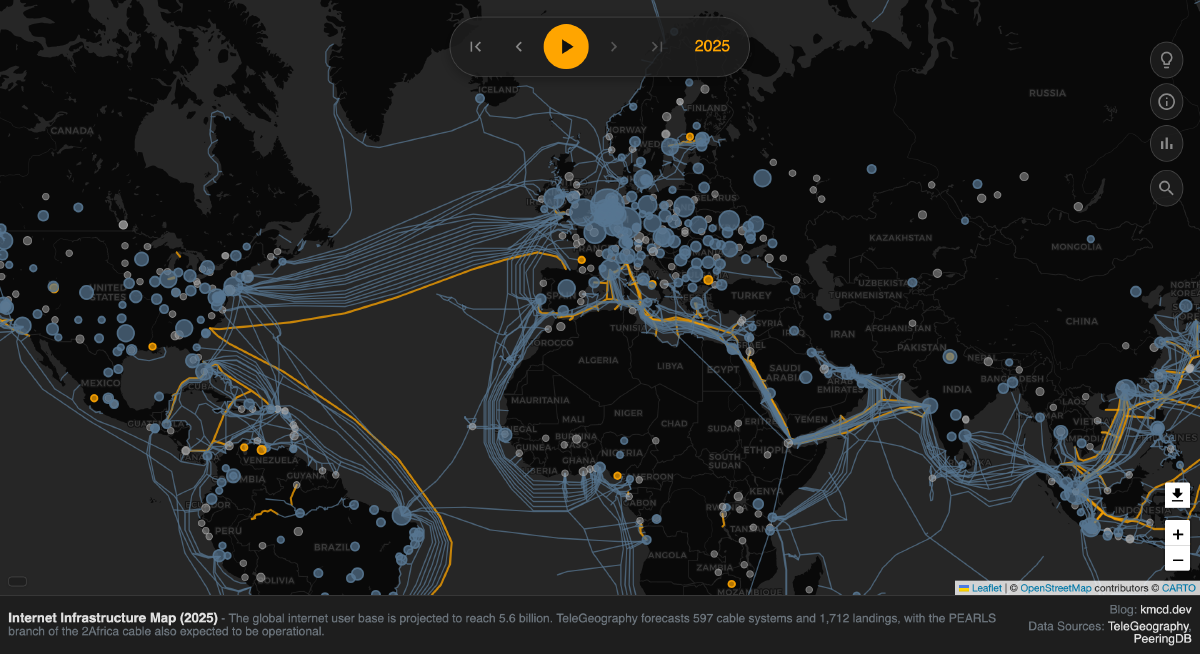
When I layered IP dominance onto the physical map, many additional cities became visible.


In earlier versions, visibility depended heavily on registered Internet Exchange Points. That highlighted the traditional coastal hubs and major peering metros. But once routing table data was incorporated, the map revealed cities without major IXPs. These are places with substantial address space and large originating networks, even if they do not host a major public exchange. This is most noticeable in India, Japan, China, Indonesia, and in secondary metros beyond traditional hubs in the EU and United States.


The physical meeting points of networks only tell us a part of the story. The global routing table reveals where address space is actually controlled and originated. Some cities carry significant weight without being major public peering hubs. The IP dominance layer makes that distinction visible.


The Chinese Internet
The Chinese internet is giant, but it presents a unique attribution challenge. Because so much of China’s domestic routing remains internal to national carriers, the global BGP table often only sees these massive networks when they peer at international hubs like Hong Kong, Los Angeles, or Frankfurt. An earlier version of my attribution code ended up adding all of China’s IP space to these select few international hubs, which was clearly incorrect. It looked like China Telecom was the biggest ISP in Germany, which made it appear that China Telecom dominated Germany. It does not, at least not yet. To fix this, I implemented specific logic for China-based networks. I used pattern matching to parse provincial hints from APNIC WHOIS data. This mapped prefixes like GD or SH to their respective provincial capitals. I also linked ASNs to their parent organizations in PeeringDB to prevent Chinese networks from being misattributed to foreign exchange points. This resolved attribution for the vast majority of prefixes. Any remaining IP space attributed only at the country level is distributed across major domestic hubs.
The result is a far more realistic view of China’s internal internet topology.
Ghost Networks and Spurious ASNs
Not every entry in the global routing table represents a real network with a physical footprint. While investigating the data, I found several “spurious” Autonomous Systems that I had to filter out to keep the map accurate.
For example, I had to add safety checks to prevent “IP swallowing.” There is a massive 0.0.0.0/0 block often pinned to Australia in the APNIC database. Since 0.0.0.0/0 matches every single IPv4 address, that one entry would incorrectly claim the entire global IP space for Australia. I know they have a lot of open space down there, but that seemed excessive.
Another prominent example was the Department of Defense (DoD). The DoD holds several massive /8 blocks (like 7.0.0.0/8 and 11.0.0.0/8). While this space is technically routed, it does not represent commercial internet traffic. In early versions of my model, the registration data for these blocks linked them to administrative offices in New York City. This caused my script to dump millions of military IPs onto Manhattan and incorrectly made it look like the absolute center of the universe.
I also built a blocklist to ignore other non-geographic entities:
- Administrative Containers: I filter out WHOIS entries containing
IANA-NETBLOCK,CIDR-BLOCK, orERX-NETBLOCK. These are typically placeholders for unassigned pools managed by regional registries rather than active networks. - Registry Placeholders: Specific ASNs like 721, 56, and 37069 often function as loopbacks or registry tests.
By explicitly ignoring these, the resulting map represents the actual commercial Internet rather than the administrative database of the Internet.
UX and Rendering
In addition to adding more data to the map, I’ve also made several improvements to the map itself.
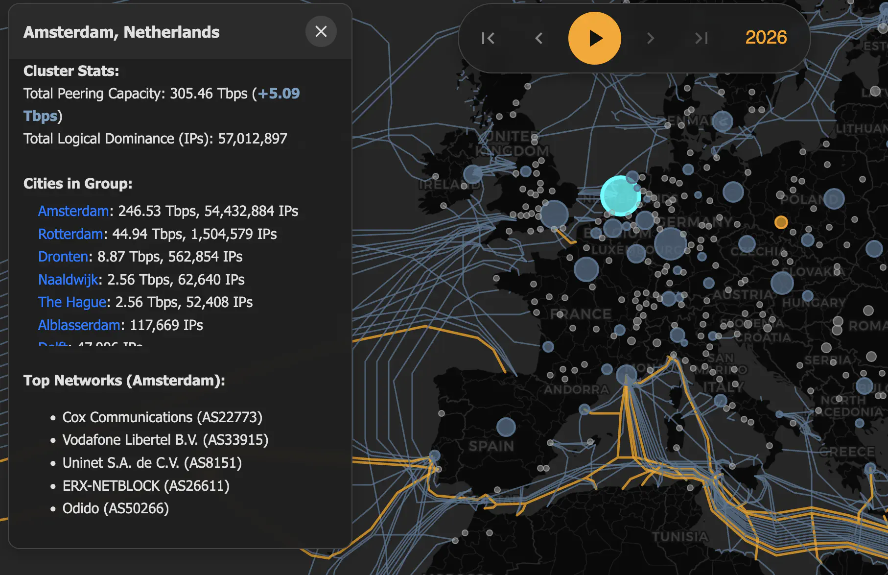
Dynamic Cluster Grouping
Layering BGP data onto an already complex physical map created a major design challenge: information density. With hundreds of new cities “lighting up” globally, the map became significantly cluttered when zoomed out.
To solve this, I implemented Dynamic Cluster Grouping. Close-by cities now group together into aggregate hubs at low zoom levels, which then split into individual markers as you zoom in. This isn’t just a visual fix; by reducing the number of active SVG shapes in the DOM, it significantly improves panning performance on mobile devices.
Dynamic Cluster Grouping ensures the map remains legible, preventing the increased data density from overwhelming the map. When you click on a cluster, the details panel expands to list every city contained within that group.
Viewport Culling
I also introduced Viewport Culling. The map now only renders assets currently within your bounds. As you pan to a new region, cities “pop in” dynamically, ensuring the browser isn’t wasting resources on rendering things on the other side of the planet.
Updates to City Sizing
The visual size of cities on the map also now dynamically reflects their importance. Previously, cities were sized based only on their relative peering bandwidth. Now, their size depends on a weighted combination of aggregate peering bandwidth and IP dominance, contributing 80% and 20% to the size calculation respectively. Although this ratio is arbitrary and was picked for aesthetic reasons, peering bandwidth is a stronger signal of real traffic concentration than raw IP space alone, so I think it should be emphasized significantly more.
Enable/disable layers
Now, the map can be sliced into three layers: Cables, peering bandwidth, and IP allocations. There are controls that allow you to show or hide each of these layers individually.

Permalinks
I also added permalinks to make the map state fully shareable. The URL now encodes the current latitude, longitude, zoom level, selected year, and active text filters. If you zoom into Southeast Asia in 2016 and search for “Singapore”, that exact view can be copied and shared. The resulting link will look like this:
https://map.kmcd.dev/?lat=3.1625&lng=103.4033&z=5.00&year=2016&q=singapore
…which will show exactly how amazingly connected Singapore is when others click on it.
Better Exports
One of the most requested features for the map has been a way to export the current view for use in presentations, reports, posters, or just as a high-quality wallpaper.
Previously, I was using a standard Leaflet plugin for this, but it was not great. It would often fail in weird ways, leaving you with a glitched or incomplete rendering of the map. It also exported as PNG, which meant the beautiful vector data of the cables and cities was flattened into a low-resolution raster format.
Now there’s a new export button that renders an isolated SVG. Because the map itself is built on SVGs, this new export method is lossless. It respects your current zoom level and position, allowing you to focus on a specific region and generate an incredibly high-quality vector file that you can scale to any size without losing a single pixel of detail. Most images in this post were generated using this new export feature.
Show Me the Data
Another one of the biggest requests I’ve had in previous years is for access to the raw data behind the visualizations. For the 2026 edition, I have exposed the underlying JSON datasets that power the map. These files are curated from TeleGeography (for modern cables), PeeringDB (for IXPs), and historical data is curated from various sources including submarinenetworks.com and archived maps.
You can access these directly to build your own visualizations, analyze the growth of global bandwidth, or double check my numbers.
all_cables.json: The Core Map Data. A GeoJSON FeatureCollection containing all submarine cables. Each feature includes properties likename,rfs_year(Ready for Service),decommission_year,owners, andlanding_points. This follows the standard GeoJSON format.year-summaries.json: Brief textual descriptions of notable events or milestones for specific years, displayed in the footer.city-dominance/{year}.json: Per-year JSON files (e.g., 2026.json) with detailed city-level peering capacity, regional information, and coordinates. Used for rendering city markers and calculating regional statistics.meta.json: Metadata including the minimum and maximum years covered by the visualization.
See You Next Year
You might ask why I burned so much time manually attributing IP space when services like MaxMind or IPInfo already exist. The honest answer? Buying the data isn’t fun. The joy of this project comes from the archaeology and the work involved in bringing order to chaotic and disjointed datasets and transforming them into something beautiful.
This was a great project, and I am extremely happy with the results. If you’ve gotten this far without checking out the map, I’m impressed with your restraint, but here’s one more link for you to take a look: Explore the Map »
About the Author

Continue the series: internet-map
- Visualizing the Internet (2022)
- Visualizing the Internet (2023)
- Visualizing the Internet (2024)
- Visualizing the Internet (2025)
- Visualizing the Internet (2026)